机器学习 - Logistic Regression
Sigmoid Function And Cost Function
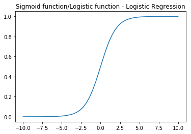
Sigmoid Function
import numpy as np
import math
x = np.linspace(-10,10);
y = 1 / (1+np.exp(-x));
from matplotlib import pyplot as plt
plt.plot(x,y,'-');
plt.title('Sigmoid function/Logistic function - Logistic Regression');
plt.show();
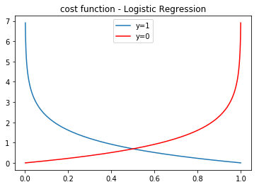
Cost Function
x = np.linspace(0.001,0.999,1000);
y = -np.log(x);
yy = -np.log(1-x);
plt.plot(x,y,x,yy,'r-');
plt.legend(["y=1","y=0"]);
plt.title('cost function - Logistic Regression')
plt.show();
Logistic Regression
build a classification model that estimates an applicant’s probability of admission based on the scores from those two exams.
读取数据
import pandas as pd
data = pd.read_csv('ex2data1.csv');
data.head()
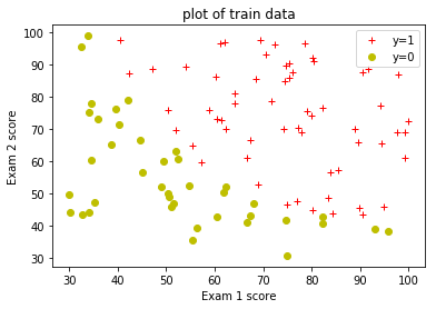
数据可视化
提取正反数据集。
positive_train_examples = data[data['admission'] == 1];
negative_train_examples = data[data['admission'] == 0];
定义绘制正反数据的辅助函数。
def plotData( x1,y1,x2,y2,
				xlabel='x',
				ylabel='y',
				title='title',
				lengend=['y=1','y=0'] ):
    plt.plot(x1,y1,'r+');
    plt.plot(x2,y2,'yo');
    plt.xlabel(xlabel);
    plt.ylabel(ylabel);
    plt.title(title);
    plt.legend(lengend,loc=1);
    plt.show();
绘制正反数据图像。
plotData( positive_train_examples['score1'],
			positive_train_examples['score2'],
			negative_train_examples['score1'],
			negative_train_examples['score2'],
        	xlabel='Exam 1 score',
			ylabel='Exam 2 score',
        	title="plot of train data" );
The Big Picture of Logistic Regression
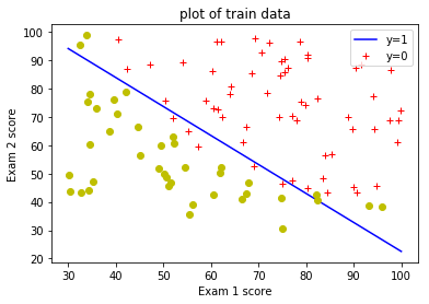
用sklearn库中的线性模型 LogisticRegression 来训练数据,得到假设函数的参数Theta。模型的准确率可以用score函数求得。而predict可以用来预测数据所属的类别,其中predict_proba可以显示概述所属类别的概率。
# https://scikit-learn.org/stable/modules/linear_model.html#logistic-regression
from sklearn.linear_model import LogisticRegression
X = data.as_matrix(['score1','score2']);
y = data['admission'];

linear_model = LogisticRegression(solver='lbfgs')
clf = linear_model.fit(X,y);
print(clf.coef_,clf.intercept_);
# out: [[0.20535491 0.2005838 ]] [-25.05219314]

clf.score(X,y)
# out: 0.89

test = [[45, 85]];
clf.predict_proba(test)
x1 = np.linspace(30,100,100);
x2 = -(clf.intercept_ + clf.coef_[0][0] * x1)/clf.coef_[0][1];
plt.plot(x1,x2,'b-');

plotData( positive_train_examples['score1'],
			positive_train_examples['score2'],
         	negative_train_examples['score1'],
			negative_train_examples['score2'],
        	xlabel='Exam 1 score',
			ylabel='Exam 2 score',
        	title="plot of train data");
Regularized logistic regression
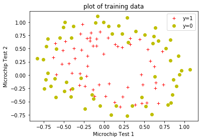
Task: predict whether microchips from a fabrication plant passes quality assurance(QA).
import pandas as pd
train_examples = pd.read_csv('ex2data2.csv');
positive_train_examples =
	train_examples[train_examples['qa']==1];
negative_train_examples =
	train_examples[train_examples['qa']==0];
数据可视化
plotData(positive_train_examples['test1'],
         positive_train_examples['test2'],
         negative_train_examples['test1'],
         negative_train_examples['test2'],
         xlabel='Microchip Test 1',
         ylabel='Microchip Test 2',
         title='plot of training data');
def mapFeatures(x1,x2):
    degree=6
    index = 0
    out = np.zeros((x1.size,27));
    out
    for i in range(1,degree+1):
        for j in range(0,i+1):
            out[:,index] = (x2 ** j) * (x1 **(i-j));
            index = index+1;
    return out

x1 = np.array([2]);
x2 = np.array([3]);
mapFeatures(x1,x2)
out: array([[ 2., 3., 4., 6., 9., 8., 12., 18., 27., 16., 24.,
36., 54., 81., 32., 48., 72., 108., 162., 243., 64., 96., 144., 216., 324., 486., 729.]])
new_X = mapFeatures(X[:,0],X[:,1]);
new_y = y;
clf = linear_model.fit(new_X,new_y);
clf.score(new_X,new_y)
out: 0.8305084745762712
print(clf.intercept_,clf.coef_);
out:
1.27271075
0.62536719
1.18095854
-2.01961804
-0.91752388
-1.43170395
0.12391867
-0.36536954
-0.35715555
-0.17501434
-1.45827831
-0.05112356
-0.61575808
-0.27472128
-1.19276292
-0.24241519
-0.20587922
-0.0448395
-0.27780311
-0.29535733
-0.45625452
-1.04347339
0.02770608
-0.29252353
0.01550105
-0.32746466
-0.1439423
-0.92460358]
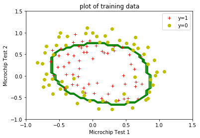
def plotDecisionBoundary(clf):
    u = np.linspace(-1,1.5,50);
    v = np.linspace(-1,1.5,50);

    U,V = np.meshgrid(u,v);
    Z = np.zeros((len(u),len(v)));
    for i in range(0,len(u)):
        for j in range(0,len(v)):
            test = mapFeatures(np.array(u[i]),np.array(v[j]));
            Z[i,j] = clf.predict(test);

    plt.contour(U,V,Z,colors='g', linewidths=1);
    plt.legend(['boundary']);

    plotData(positive_train_examples['test1'],
         positive_train_examples['test2'],
         negative_train_examples['test1'],
         negative_train_examples['test2'],
         xlabel='Microchip Test 1',
         ylabel='Microchip Test 2',
         title='plot of training data');

plotDecisionBoundary(clf);
Multi-class logistic Regression
extract training data into csv format
load('ex3data1.mat')
m = [X, y];
csvwrite('handwritten_digits.csv',m);
read training data
import pandas as pd
train_data  = pd.read_csv('handwritten_digits.csv',header=None)
train_data.head()
preprocess training data into X, y
import numpy as np
index = list(range(0,400))
X = train_data.as_matrix(index);
y = train_data[400];
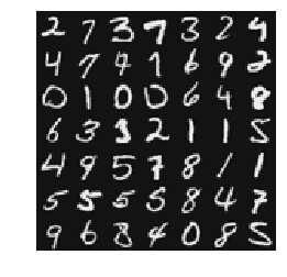
visualize training data in graphic mode
from matplotlib import pyplot as plt
def displayData(X,row=None,col=None):
    m,n=X.shape
    w = h = int(np.sqrt(n))
    if row==None or col == None:
        row = col = int(np.sqrt(m))
    data = []
    index = 0
    for r in range(0,row):
        rows = []
        for c in range(0,col):
            rows.append(np.reshape(X[index,:],(w,h),order='F'))
            index = index + 1
        data.append(rows)

    rows = []
    for r in range(0,row):
        t = np.concatenate(tuple(data[r]),axis=1);
        rows.append(t);

    c = np.concatenate(tuple(rows));
    plt.imshow(c,cmap="gray")
    plt.axis('off')
    plt.show();

m,n=X.shape
rand_indice = np.random.permutation(m)
displayData(X[rand_indice[:49]]);
train the model
from sklearn.linear_model import LogisticRegression
linear_model = LogisticRegression(solver='lbfgs')
clf = linear_model.fit(X,y);
print("Training Set Accuracy: ",clf.score(X,y))
Training Set Accuracy: 0.9446
predict train data
m,n=X.shape
rand_indice = np.random.permutation(m)
row=4
col=3
test_train = X[rand_indice[:row*col]]
displayData(test_train,row,col)
print(np.reshape(clf.predict(test_train),(row,col)))
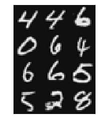
[
[ 4 4 6]
[10 6 4]
[ 6 6 5]
[ 5 2 8]
]